Diffusion-Based Generative Models <3>: SMLD

July 10, 2025

一. 引言

在生成模型的研究中，基于得分（Score-based）的生成方法提供了一种从目标分布生成数据的新颖而强大的框架。与传统的生成方法不同，这类模型通过估计数据分布的梯度信息——即所谓的得分函数 (Stein’s) score function，来指导样本生成过程。

其核心思想在于利用统计物理学中的朗之万动力学（Langevin Dynamics）作为采样工具，将随机噪声逐步演化为符合目标分布的样本。

尽管在一维情况下，我们可以通过反累积分布函数（CDF）的方法轻松实现采样，但在高维空间中，这种直接方法不再适用。此时，Score-based的方法则展现出其独特优势：它通过对概率密度的局部变化进行建模，使得生成过程能够在计算上变得可行，并赋予模型更强的表达能力和灵活性。

本部分将介绍(Denosing) Score Matching，并通过 Langevin Dynamics进行采样的算法思想。最后给出SMLD (Score Matching with Langevin Dynamics)的算法框架。

二. 背景

2.1 一维变量的采样

考虑一种简单情况，$ x \in \mathbb{R}^1 $ 为一维变量，$ x \sim p(x)$，可以通过逆变换采样（Inverse Transform Sampling），从 $ p(x)$进行随机采样，求其累计密度函数 CDF：

$$ F(x) = p(X \leq x) $$

然后求CDF的逆函数，并从 $[0,1]$ 均匀分布中采样, 代入到CDF的逆函数中，就能实现从分布 $ p(x)$ 中采样：

$$ \begin{aligned} u &\sim Uniform[0,1] \\ x &= F^{-1}(u) \end{aligned} $$

（再回想下VAE中的Reparameterization技巧，从高斯分布 $\mathcal{N}(\mu, \sigma^2)$ 中采样时，是先从标准正态分布 $\mathcal{N}(0, 1)$ 中采样得到 $\mathbf{\epsilon}$，然后通过变换 $x = \mu + \sigma \epsilon$ 得到样本。VAE采用这种技巧的主要目的是解决反向传播时梯度无法通过随机采样节点的问题）

但对于高维变量来说，这种方法是行不通的：

在高维空间中，计算CDF变得极其困难：CDF变成 $F(x_1, x_2, …, x_d) = \int_{-\infty}^{x_1} \int_{-\infty}^{x_2} … \int_{-\infty}^{x_d} p(t_1, t_2, …, t_d) dt_1 dt_2 … dt_d$，这个多重积分的计算复杂度随维度呈指数增长。
即使能够计算出高维CDF，其逆函数 $F^{-1}(u_1, u_2, …, u_d)$ 的求解也极其困难，通常是没有解析解的。
高维空间中数据分布的稀疏性问题，这是所有生成式模型面临的共同挑战。

2.2 Langevin Dynamics

如何对高维空间的变量进行采样呢，有效地采样意味着我们希望从概率密度更高的地方进行采样，如果有 $ p(\mathbf{x})$ 的梯度，那就可以根据梯度前往高密度区域采样。等价地假设有 $ \log p(\mathbf{x})$ 的梯度 $ \nabla_{\mathbf{x}} \log p(\mathbf{x})$，这里使用 $ \nabla_{\mathbf{x}} \log p(\mathbf{x})$ 的原因是$\log p(\mathbf{x})$ 的梯度在数值上更稳定，梯度方向相同，在采样过程中，我们关心的是梯度方向，而不是梯度大小。

为了简化表示，我们将 $\nabla_{\mathbf{x_t}} \log p(\mathbf{x_{t}})$ 记为 $\nabla_{\mathbf{x}} \log p_t(\mathbf{x})$。通过梯度上升方法，可以迭代更新样本位置：

$$ \mathbf{x_{t+1}} = \mathbf{x_{t}} + \tau \nabla_{\mathbf{x}} \log p_t(\mathbf{x}) $$

其中 $\tau > 0$ 是步长参数，控制每次更新的幅度。然而，这种纯梯度上升方法存在一个根本性问题：样本最终会收敛到概率密度的局部最大值点，无法实现对整个目标分布的采样。

为了实现真正的从分布 $p(\mathbf{x})$ 中采样，我们需要引入朗之万动力学（Langevin Dynamics），这是一种基于马尔可夫链蒙特卡罗（MCMC）的采样方法。该方法在梯度上升的基础上添加随机噪声项：

$$ \mathbf{x_{t+1}} = \mathbf{x_{t}} + \tau \nabla_{\mathbf{x}} \log p_t(\mathbf{x}) + \sqrt{2\tau} \mathbf{z}_t, \quad t = 0, 1, \dots, T-1 $$

其中：

$\tau$ 是步长参数，控制更新步长的大小
$\mathbf{z}_t \sim \mathcal{N}(\mathbf{0}, \mathbf{I})$ 是独立同分布的高斯噪声
$T$ 是总迭代次数，决定了采样过程的长度
$\sqrt{2\tau}$ 是噪声的标准差，这个特定选择确保了在 $\tau \to 0$ 时，离散时间过程收敛到连续时间的朗之万扩散过程

$\tau$ 和 $T$ 的关系：较小的 $\tau$ 值需要更大的 $T$ 值来确保采样过程充分探索目标分布。通常选择 $\tau$ 使得 $T \cdot \tau$ 保持在一个合理的范围内，以保证采样效率和收敛性。

对比可以发现

$$ Langevin \ Dynamics = gradient \ descent/ascent + noise $$

梯度上升是告诉我们如何找到局部最大值点($p(\mathbf{x}的峰值)$)，而Langevin Dynamics告诉我们如何从 $p(\mathbf{x})$ 采样。

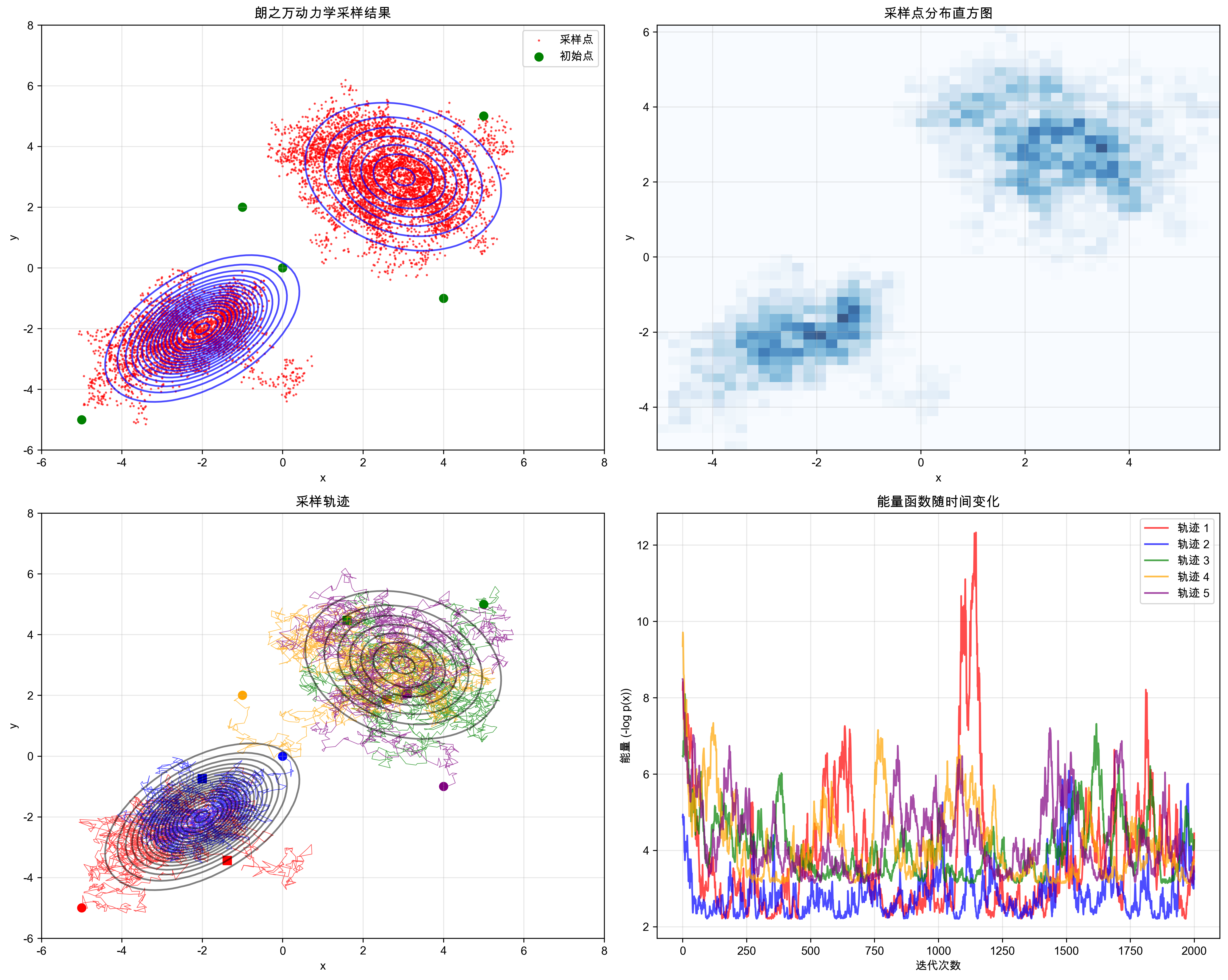
给GPT一个简单prompt，可以模拟在二维混合高斯分布上迭代Langevin Dynamic的效果:

2.3 Score Matching

2.3.1 (Stein’s) Score Function

在Autoregressive models/Variational autoencoder/Energy based models/Normalizing flow等Likelihood-based model中，都是对 $p(\mathbf{x})$ 进行建模，给定 $\theta$ 为模型可学习参数，可以定义PDF为：

$$ p_{\theta}(\mathbf{x}) = \frac{\exp^{-f_{\theta}(\mathbf{x})}}{Z_{\theta}} $$

其中，$f_{\theta}(\mathbf{x})$ 为未归一化的概率模型（unnormalized probabilistic model），也称为基于能量的模型（energy-based model），$Z_{\theta}$ 为归一化常数（normalization constant），定义为：

$$ Z_{\theta} = \int \exp^{-f_{\theta}(\mathbf{x})} d\mathbf{x} $$

这个积分确保PDF满足 $\int p_{\theta}(\mathbf{x}) d\mathbf{x} = 1$ 的归一化条件。

在基于得分的生成模型中，我们通常不直接建模 $\nabla_{\mathbf{x}} p_{\theta}(\mathbf{x})$，而是建模得分函数(Stein’s) score function $\nabla_{\mathbf{x}} \log p_{\theta}(\mathbf{x})$，从而避免计算复杂的归一化常数 $Z_{\theta}$。

$Z_{\theta}$补充

为什么避免 $Z_{\theta}$ 很重要：

计算困难：对于高维数据，$Z_{\theta}$ 的计算涉及高维积分，计算复杂度呈指数增长
数值不稳定：直接计算 $Z_{\theta}$ 在数值上不稳定，容易出现上溢或下溢
模型灵活性：通过建模得分函数，我们可以使用任意的能量函数 $f_{\theta}(\mathbf{x})$，而不需要确保其积分收敛

为什么 $Z_{\theta}$ 对 $\mathbf{x}$ 求导为0：

归一化常数 $Z_{\theta} = \int \exp^{-f_{\theta}(\mathbf{x})} d\mathbf{x}$ 是一个与 $\mathbf{x}$ 无关的常数，因为：

积分变量：$Z_{\theta}$ 中的积分变量是 $\mathbf{x}$，积分后得到的是一个标量常数
参数独立性：$Z_{\theta}$ 只依赖于模型参数 $\theta$，不依赖于具体的 $\mathbf{x}$ 值
数学性质：对于任意常数 $c$，有 $\nabla_{\mathbf{x}} c = 0$

因此：

$$ \nabla_{\mathbf{x}} \log p_{\theta}(\mathbf{x}) = \nabla_{\mathbf{x}} \log \frac{\exp^{-f_{\theta}(\mathbf{x})}}{Z_{\theta}} = \nabla_{\mathbf{x}} (-f_{\theta}(\mathbf{x}) - \log Z_{\theta}) = -\nabla_{\mathbf{x}} f_{\theta}(\mathbf{x}) $$

这就是为什么基于得分的方法可以避免计算 $Z_{\theta}$ 的原因。

构建一个基于分数的模型 $s_\theta(\mathbf{x}) = \nabla_{\mathbf{x}} \log p_{\theta}(\mathbf{x})$，通过最小化模型学习分布和真实分布的Fisher散度:

$$ \frac{1}{2} \mathbb{E}_{p(\mathbf{x})} \left[ \| \nabla_{\mathbf{x}} \log p({\mathbf{x}}) - s_\theta(\mathbf{x})\|_2^2 \right] $$

但直接计算上式子是不可行的，显然我们无法得知 $\nabla_{\mathbf{x}} \log p({\mathbf{x}})$。

Score Matching解决的就是这个问题。Score Matching最早是由 Estimation of Non-Normalized Statistical Models by Score Matching 这篇文章所提出，通过分部积分法来规避无法计算的 $\nabla_{\mathbf{x}} \log p({\mathbf{x}})$。

2.3.2 Score Matching 的数学推导

展开上式，可以将Fisher散度转换为：

$$ \begin{aligned} &\frac{1}{2} \mathbb{E}_{p(\mathbf{x})} \left[ \| \nabla_{\mathbf{x}} \log p({\mathbf{x}}) - s_\theta(\mathbf{x})\|_2^2 \right] \\ = &\frac{1}{2} \mathbb{E}_{p(\mathbf{x})} \left[ \| \nabla_{\mathbf{x}} \log p({\mathbf{x}})\|_2^2 \right] + \frac{1}{2} \mathbb{E}_{p(\mathbf{x})} \left[ \| s_\theta(\mathbf{x})\|_2^2 \right] - \mathbb{E}_{p(\mathbf{x})} \left[ (\nabla_{\mathbf{x}} \log p({\mathbf{x}}))^T s_\theta(\mathbf{x}) \right] \end{aligned} $$

其中第一项与模型参数 $\theta$ 无关，可以忽略。对于第三项，通过分部积分可以得到：

$$ \mathbb{E}_{p(\mathbf{x})} \left[ (\nabla_{\mathbf{x}} \log p({\mathbf{x}}))^T s_\theta(\mathbf{x}) \right] = -\mathbb{E}_{p(\mathbf{x})} \left[ \text{tr}(\nabla_{\mathbf{x}} s_\theta(\mathbf{x})) \right] $$

第三项分部积分的推导

对于任意标量函数 $f(\mathbf{x})$ 和 $g(\mathbf{x})$，在 $\mathbb{R}^d$ 上，如果 $f(\mathbf{x})g(\mathbf{x}) \to 0$ 当 $ ||\mathbf{x}|| \to \infty $，则有：

$$ \int \nabla_{\mathbf{x}} f(\mathbf{x}) g(\mathbf{x}) d\mathbf{x} = -\int \nabla_{\mathbf{x}} g(\mathbf{x}) f(\mathbf{x}) d\mathbf{x} $$

推广到标量函数 $f(\mathbf{x})$ 和向量场 $\mathbf{g}(\mathbf{x})$，则有：

$$ \int (\nabla_{\mathbf{x}} f(\mathbf{x}))^T \mathbf{g}(\mathbf{x}) d\mathbf{x} = -\int f(\mathbf{x}) \nabla_{\mathbf{x}} \cdot \mathbf{g}(\mathbf{x}) d\mathbf{x} $$

应用到我们的情况：

$$ \begin{aligned} \mathbb{E}_{p(\mathbf{x})} \left[ (\nabla_{\mathbf{x}} \log p({\mathbf{x}}))^T s_\theta(\mathbf{x}) \right] &= \int p(\mathbf{x}) (\nabla_{\mathbf{x}} \log p({\mathbf{x}}))^T s_\theta(\mathbf{x}) d\mathbf{x} \\ &= \int (\nabla_{\mathbf{x}} p({\mathbf{x}}))^T s_\theta(\mathbf{x}) d\mathbf{x} \\ &= -\int p(\mathbf{x}) \nabla_{\mathbf{x}} \cdot s_\theta(\mathbf{x}) d\mathbf{x} \quad \text{(分部积分)} \\ &= -\mathbb{E}_{p(\mathbf{x})} \left[ \text{tr}(\nabla_{\mathbf{x}} s_\theta(\mathbf{x})) \right] \end{aligned} $$

$p(\mathbf{x})$ 是标量函数（概率密度）
$s_\theta(\mathbf{x})$ 是向量场（得分函数，维度与 $\mathbf{x}$ 相同）

其中 $\nabla_{\mathbf{x}} \cdot s_\theta(\mathbf{x}) = \text{tr}(\nabla_{\mathbf{x}} s_\theta(\mathbf{x}))$ 是向量场的散度。

因此，Score Matching的目标函数变为：

$$ \mathcal{L}(\theta) = \frac{1}{2} \mathbb{E}_{p(\mathbf{x})} \left[ \| s_\theta(\mathbf{x})\|_2^2 + 2 \text{tr}(\nabla_{\mathbf{x}} s_\theta(\mathbf{x})) \right] $$

但是目标函数中 $\text{tr}(\nabla_{\mathbf{x}} s_\theta(\mathbf{x}))$ 这一项，$ s_\theta(\mathbf{x})$ 是与输入维度相同的得分函数，对高维数据来说，其雅可比矩阵迹的计算成本极高，很难直接求解。

PyTorch自动微分机制下计算雅可比矩阵迹的成本

在Score Matching的目标函数中，我们需要计算 $\text{tr}(\nabla_{\mathbf{x}} s_\theta(\mathbf{x}))$，即得分函数 $s_\theta(\mathbf{x}) \in \mathbb{R}^n$ 对输入 $\mathbf{x} \in \mathbb{R}^n$ 的雅可比矩阵的迹。在PyTorch的自动微分机制下，这个计算过程存在显著的计算和内存开销。

自动微分的底层行为

PyTorch在计算雅可比矩阵时，会按以下步骤进行：

前向传播：计算 $s_\theta(\mathbf{x}) \in \mathbb{R}^n$。

反向传播：

对输出向量的每个分量 $[s_\theta(\mathbf{x})]_i$：
- 调用 torch.autograd.grad 计算其梯度 $\nabla[s_\theta(\mathbf{x})]_i \in \mathbb{R}^n$
- 将结果存储为雅可比矩阵的第 $i$ 行
重复 $n$ 次，得到完整的雅可比矩阵 $J \in \mathbb{R}^{n \times n}$

计算图与内存开销

存储复杂度：显式存储雅可比矩阵 $J$ 需要 $O(n^2)$ 内存。

计算复杂度：需执行 $n$ 次独立的反向传播，每次计算 $\mathbb{R}^n$ 梯度，总复杂度 $O(n^2)$。

中间层的雅可比信息

局部雅可比矩阵：每个线性层 $y = Wx + b$ 的雅可比是权重矩阵 $W$。

非线性层（如ReLU）：雅可比是对角矩阵，对角线元素为激活函数的导数。

链式法则：全局雅可比 $J$ 是各层局部雅可比的乘积，但PyTorch不会显式存储中间结果。

针对雅可比矩阵的迹，有以下几种高效计算方案：

$$\text{tr}(J) \approx \mathbb{E}[v^T J v] = \mathbb{E}[v^T \nabla(s_\theta(\mathbf{x})^T v)]$$
Sliced Score Matching：避免计算迹，通过随机投影简化目标函数
Denoising Score Matching：通过添加噪声避免迹的计算

2.3.3 Score Matching的根本性问题：低密度区域的估计困难

尽管Score Matching提供了一种避免计算雅可比矩阵迹的方法，但它仍然面临一个根本性的挑战：在高维空间中，数据分布呈现出严重的稀疏性，导致低密度区域的得分函数估计极其困难。

高维空间的稀疏性

维度诅咒（Curse of Dimensionality）：

在高维空间中，数据点之间的距离变得不直观
随着维度增加，数据分布变得越来越稀疏
大部分空间区域都是"空"的，没有训练数据

稀疏性的数学表现：对于 $d$ 维空间中的单位超立方体 $[0,1]^d$：

体积：$V = 1^d = 1$
但数据主要集中在极小的子空间中
大部分区域的概率密度 $p(\mathbf{x}) \approx 0$

对得分函数估计的影响：

训练数据不足：低密度区域缺乏训练样本
梯度信息缺失：$\nabla_{\mathbf{x}} \log p(\mathbf{x})$ 在低密度区域无法准确估计
模型泛化困难：神经网络难以在未见过的区域做出准确预测

朗之万动力学采样的关键问题：

当使用朗之万动力学进行采样时，初始样本 $\mathbf{x}_0$ 通常来自随机噪声分布（如标准正态分布），这意味着：

初始位置问题：$\mathbf{x}_0$ 极有可能位于低密度区域
错误引导：如果得分函数 $s_\theta(\mathbf{x})$ 在低密度区域估计不准确，整个采样过程从一开始就会被误导
质量下降：错误的梯度信息会导致生成的样本质量差，无法代表真实数据分布

解决方案的动机：

为了克服低密度区域得分函数估计不准确的问题，下面介绍一种高效方式 Denoising Score Matching：通过添加噪声，将低密度区域"填充"为高密度区域

2.4 Denoising Score Matching

$$ \mathcal{L}_{ESM_{p_0}}(\theta) =\frac{1}{2} \mathbb{E}_{p_0(\mathbf{x})} \left[ \| \nabla_{\mathbf{x}} \log p_0({\mathbf{x}}) - s_\theta(\mathbf{x})\|_2^2 \right] $$

表示从真实分布 $p(\mathbf{x}) = p_0(\mathbf{x})$ 中进行采样的目标函数。

通过加高斯噪声的方式，对 $\mathbf{x}$ 施加扰动得到 $\tilde{\mathbf{x}}$ ：

$$ \tilde{\mathbf{x}} = \mathbf{x} + \sigma \mathbf{z} , \quad z \sim \mathcal{N}(0, \mathbf{I}) $$

扩展原目标函数：

$$ \mathcal{L}_{ESM_{p_\sigma}}(\theta) =\frac{1}{2} \mathbb{E}_{p_\sigma(\tilde{\mathbf{x}})} \left[ \| \nabla_{\tilde{\mathbf{x}}} \log p_\sigma({\tilde{\mathbf{x}}}) - s_\theta(\tilde{\mathbf{x}})\|_2^2 \right] $$

这里 $p_\sigma(\tilde{\mathbf{x}})$ 表示的是扰动后的数据分布。很显然，在上式目标函数中，学习的是扰动后的数据分布信息。

这里是我觉得很有意思的一点：Denoising Score Matching（DSM）的核心本质并不是直接学习真实数据分布 $p_0(\mathbf{x})$ 的得分函数，而是学习加噪后分布 $p_\sigma(\tilde{\mathbf{x}})$ 的得分函数。只有当噪声 $\sigma \to 0$ 时，DSM 学到的得分函数才会逼近真实分布的得分函数。

上式是DSM希望学习的目标，可惜上式也无法直接求解析解，因为 $p_\sigma(\tilde{\mathbf{x}})$ 的解析形式仍不可知。不过我们知道 $p_\sigma(\tilde{\mathbf{x}} | \mathbf{x}) $ 是有解析解的，因为扰动尺度 $\sigma$ 是已知的超参数。

对不同的噪声尺度 $\sigma$，定义新的目标函数：

$$ \mathcal{L}_{DSM_{p_\sigma}}(\theta) = \frac{1}{2} \mathbb{E}_{p_\sigma(\mathbf{x}, \tilde{\mathbf{x}})} \left[ \| s_\theta(\mathbf{\tilde{\mathbf{x}}}) - \nabla_{\tilde{\mathbf{x}}} \log p({\tilde{\mathbf{x}}} | \mathbf{x}) \|_2^2 \right] $$

添加噪声后，$\tilde{\mathbf{x}}$ 的分布为：

$$ p_\sigma(\tilde{\mathbf{x}} | \mathbf{x}) = \frac{1}{(2\pi\sigma^2)^{d/2}} \exp\left(-\frac{\|\tilde{\mathbf{x}} - \mathbf{x}\|_2^2}{2\sigma^2}\right) $$

其中 $d$ 是数据维度。因此：

$$ \log p_\sigma(\tilde{\mathbf{x}} | \mathbf{x}) = -\frac{d}{2}\log(2\pi\sigma^2) - \frac{\|\tilde{\mathbf{x}} - \mathbf{x}\|_2^2}{2\sigma^2} $$

对 $\tilde{\mathbf{x}}$ 求梯度：

$$ \nabla_{\tilde{\mathbf{x}}} \log p_\sigma(\tilde{\mathbf{x}} | \mathbf{x}) = -\frac{\tilde{\mathbf{x}} - \mathbf{x}}{\sigma^2} = -\frac{\mathbf{z}}{\sigma} $$

其中 $\mathbf{z} = \frac{\tilde{\mathbf{x}} - \mathbf{x}}{\sigma} \sim \mathcal{N}(0, \mathbf{I})$。

代入目标函数：

$$ \begin{aligned} \mathcal{L}_{DSM_{p_\sigma}}(\theta) &= \frac{1}{2} \mathbb{E}_{p_\sigma(\mathbf{x}, \tilde{\mathbf{x}})} \left[ \| s_\theta(\tilde{\mathbf{x}}) - \nabla_{\tilde{\mathbf{x}}} \log p_\sigma(\tilde{\mathbf{x}} | \mathbf{x}) \|_2^2 \right] \\ &= \frac{1}{2} \mathbb{E}_{p_\sigma(\mathbf{x}, \tilde{\mathbf{x}})} \left[ \| s_\theta(\tilde{\mathbf{x}}) + \frac{\mathbf{z}}{\sigma} \|_2^2 \right] \\ % &= \frac{1}{2} \mathbb{E}_{p_0(\mathbf{x})} \int p(\tilde{\mathbf{x}} | \mathbf{x}) \left[ \| s_\theta(\tilde{\mathbf{x}}) + \frac{\mathbf{z}}{\sigma} \|_2^2 \right] d \tilde{\mathbf{x}} \end{aligned} $$

完美！可以根据目标函数的解析形式来学习得分函数 $s_\theta(\tilde{\mathbf{x}})$ 了，但在此之前，还需要证明一个关键问题：

$$\mathcal{L}_{DSM_{p_\sigma}}(\theta) \quad 和 \quad \mathcal{L}_{ESM_{p_\sigma}}(\theta) \quad 的等价性$$

DSM与ESM目标函数的等价性证明

我们需要证明：

$$ \mathcal{L}_{DSM_{p_\sigma}}(\theta) = \mathcal{L}_{ESM_{p_\sigma}}(\theta) + C $$

其中 $C$ 是与 $\theta$ 无关的常数。

直观理解：

让我们直接展开两个目标函数，看看它们的结构：

$$ \begin{aligned} \mathcal{L}_{ESM_{p_\sigma}}(\theta) &= \frac{1}{2} \mathbb{E}_{p_\sigma(\tilde{\mathbf{x}})} \left[ \| \nabla_{\tilde{\mathbf{x}}} \log p_\sigma(\tilde{\mathbf{x}}) - s_\theta(\tilde{\mathbf{x}})\|_2^2 \right] \\ &= \frac{1}{2} \mathbb{E}_{p_\sigma(\tilde{\mathbf{x}})} \left[ \| s_\theta(\tilde{\mathbf{x}}) \|_2^2 \right] + \frac{1}{2} \mathbb{E}_{p_\sigma(\tilde{\mathbf{x}})} \left[ \| \nabla_{\tilde{\mathbf{x}}} \log p_\sigma(\tilde{\mathbf{x}}) \|_2^2 \right] \\ &\quad - \mathbb{E}_{p_\sigma(\tilde{\mathbf{x}})} \left[ (\nabla_{\tilde{\mathbf{x}}} \log p_\sigma(\tilde{\mathbf{x}}))^T s_\theta(\tilde{\mathbf{x}}) \right] \end{aligned} $$$$ \begin{aligned} \mathcal{L}_{DSM_{p_\sigma}}(\theta) &= \frac{1}{2} \mathbb{E}_{p_\sigma(\mathbf{x}, \tilde{\mathbf{x}})} \left[ \| s_\theta(\tilde{\mathbf{x}}) - \nabla_{\tilde{\mathbf{x}}} \log p_\sigma(\tilde{\mathbf{x}} | \mathbf{x}) \|_2^2 \right] \\ &= \frac{1}{2} \mathbb{E}_{p_\sigma(\tilde{\mathbf{x}})} \left[ \| s_\theta(\tilde{\mathbf{x}}) \|_2^2 \right] + \frac{1}{2} \mathbb{E}_{p_\sigma(\mathbf{x}, \tilde{\mathbf{x}})} \left[ \| \nabla_{\tilde{\mathbf{x}}} \log p_\sigma(\tilde{\mathbf{x}} | \mathbf{x}) \|_2^2 \right] \\ &\quad - \mathbb{E}_{p_\sigma(\mathbf{x}, \tilde{\mathbf{x}})} \left[ s_\theta(\tilde{\mathbf{x}})^T \nabla_{\tilde{\mathbf{x}}} \log p_\sigma(\tilde{\mathbf{x}} | \mathbf{x}) \right] \end{aligned} $$

对比俩个目标函数展开后的形式容易发现：第一项相同；第二项与 $\theta无关$ 为常数；我们只需要证明第三项的等价性：

$$ \mathbb{E}_{p_\sigma(\tilde{\mathbf{x}})} \left[ (\nabla_{\tilde{\mathbf{x}}} \log p_\sigma(\tilde{\mathbf{x}}))^T s_\theta(\tilde{\mathbf{x}}) \right] = \mathbb{E}_{p_\sigma(\mathbf{x}, \tilde{\mathbf{x}})} \left[ s_\theta(\tilde{\mathbf{x}})^T \nabla_{\tilde{\mathbf{x}}} \log p_\sigma(\tilde{\mathbf{x}} | \mathbf{x}) \right] $$

详细推导：

$$ \begin{aligned} &\quad \mathbb{E}_{p_\sigma(\tilde{\mathbf{x}})} \left[ s_\theta(\tilde{\mathbf{x}})^T \nabla_{\tilde{\mathbf{x}}} \log p_\sigma(\tilde{\mathbf{x}}) \right] \\ &= \int_{\tilde{\mathbf{x}}} p_\sigma(\tilde{\mathbf{x}}) \left\langle s_\theta(\tilde{\mathbf{x}}), \nabla_{\tilde{\mathbf{x}}} \log p_\sigma(\tilde{\mathbf{x}}) \right\rangle d\tilde{\mathbf{x}} \\ &= \int_{\tilde{\mathbf{x}}} p_\sigma(\tilde{\mathbf{x}}) \left\langle s_\theta(\tilde{\mathbf{x}}), \frac{\nabla_{\tilde{\mathbf{x}}} p_\sigma(\tilde{\mathbf{x}})}{p_\sigma(\tilde{\mathbf{x}})} \right\rangle d\tilde{\mathbf{x}} \\ &= \int_{\tilde{\mathbf{x}}} \left\langle s_\theta(\tilde{\mathbf{x}}), \nabla_{\tilde{\mathbf{x}}} p_\sigma(\tilde{\mathbf{x}}) \right\rangle d\tilde{\mathbf{x}} \\ &= \int_{\tilde{\mathbf{x}}} \left\langle s_\theta(\tilde{\mathbf{x}}), \nabla_{\tilde{\mathbf{x}}} \int_{\mathbf{x}} p_0(\mathbf{x}) p_\sigma(\tilde{\mathbf{x}} | \mathbf{x}) d\mathbf{x} \right\rangle d\tilde{\mathbf{x}} \\ &= \int_{\tilde{\mathbf{x}}} \left\langle s_\theta(\tilde{\mathbf{x}}), \int_{\mathbf{x}} p_0(\mathbf{x}) \nabla_{\tilde{\mathbf{x}}} p_\sigma(\tilde{\mathbf{x}} | \mathbf{x}) d\mathbf{x} \right\rangle d\tilde{\mathbf{x}} \\ &= \int_{\tilde{\mathbf{x}}} \left\langle s_\theta(\tilde{\mathbf{x}}), \int_{\mathbf{x}} p_0(\mathbf{x}) p_\sigma(\tilde{\mathbf{x}} | \mathbf{x}) \nabla_{\tilde{\mathbf{x}}} \log p_\sigma(\tilde{\mathbf{x}} | \mathbf{x}) d\mathbf{x} \right\rangle d\tilde{\mathbf{x}} \\ &= \int_{\tilde{\mathbf{x}}} \int_{\mathbf{x}} p_0(\mathbf{x}) p_\sigma(\tilde{\mathbf{x}} | \mathbf{x}) \left\langle s_\theta(\tilde{\mathbf{x}}), \nabla_{\tilde{\mathbf{x}}} \log p_\sigma(\tilde{\mathbf{x}} | \mathbf{x}) \right\rangle d\mathbf{x} d\tilde{\mathbf{x}} \\ &= \int_{\tilde{\mathbf{x}}} \int_{\mathbf{x}} p_\sigma(\tilde{\mathbf{x}}, \mathbf{x}) \left\langle s_\theta(\tilde{\mathbf{x}}), \nabla_{\tilde{\mathbf{x}}} \log p_\sigma(\tilde{\mathbf{x}} | \mathbf{x}) \right\rangle d\mathbf{x} d\tilde{\mathbf{x}} \\ &= \mathbb{E}_{p_\sigma(\mathbf{x}, \tilde{\mathbf{x}})} \left[ s_\theta(\tilde{\mathbf{x}})^T \nabla_{\tilde{\mathbf{x}}} \log p_\sigma(\tilde{\mathbf{x}} | \mathbf{x}) \right] \end{aligned} $$

通过上述推导，我们证明了ESM和DSM目标函数中的交叉项相等，因此两个目标函数只相差一个与 $\theta$ 无关的常数项，在优化意义上等价。

因此，我们不需要计算雅可比矩阵迹，可以使用该目标来训练模型：

$$ \begin{aligned} \mathcal{L}_{DSM_{p_\sigma}}(\theta) &= \frac{1}{2} \mathbb{E}_{p_\sigma(\mathbf{x}, \tilde{\mathbf{x}})} \left[ \| s_\theta(\tilde{\mathbf{x}}) + \frac{\mathbf{z}}{\sigma} \|_2^2 \right] \\ % &= \frac{1}{2} \mathbb{E}_{p_0(\mathbf{x})} \int p(\tilde{\mathbf{x}} | \mathbf{x}) \left[ \| s_\theta(\tilde{\mathbf{x}}) + \frac{\mathbf{z}}{\sigma} \|_2^2 \right] d \tilde{\mathbf{x}} \end{aligned} $$

关于DSM，有两个核心要点值得强调：

DSM的核心思想是通过添加噪声来解决Score Matching在高维数据稀疏性区域估计困难的问题。
DSM并非直接学习真实数据分布 $p_0(\mathbf{x})$ 的得分函数，而是学习加噪后分布 $p_\sigma(\tilde{\mathbf{x}})$ 的得分函数。只有当噪声尺度 $\sigma \to 0$ 时，DSM学到的得分函数才会逼近真实分布的得分函数。但观察上述目标函数不难发现，当 $\sigma \to 0$ 时，会存在数值不稳定的问题。

综上，DSM不仅为下文的SMLD方法提供了理论基础，也与后续基于ODE/SDE的Diffusion Model及Flow Matching等生成模型方法密切相关。

三. SMLD算法框架

有了上面的铺垫，介绍SMLD(Score Matching with Langevin Dynamics)的算法框架就变得清晰了。这里主要介绍SMLD的具体实现方法：NCSN（Noise Conditioned Score Network），核心思想包含两个关键点：

多尺度噪声扰动：使用不同尺度的噪声 ${\sigma_1, \sigma_2, …, \sigma_L}$ 对数据进行扰动，其中 $\sigma_1 > \sigma_2 > … > \sigma_L$。较大尺度的噪声能够更好地填充高维数据稀疏区域，而较小尺度的噪声则能更好地逼近真实数据分布 $p_0(\mathbf{x})$。
MCMC采样：训练得到多尺度得分函数 $s_\theta(\mathbf{x}, \sigma_i)$ 后，利用Langevin Dynamics从大尺度噪声开始，逐步向小尺度噪声采样，最终生成高质量样本。

3.1 多尺度噪声扰动

对于每个噪声尺度 $\sigma_i$，我们定义扰动后的数据分布：

$$ p_{\sigma_i}(\tilde{\mathbf{x}}) = \int p_0(\mathbf{x}) p_{\sigma_i}(\tilde{\mathbf{x}} | \mathbf{x}) d\mathbf{x} $$

其中条件分布为：

$$ p_{\sigma_i}(\tilde{\mathbf{x}} | \mathbf{x}) = \frac{1}{(2\pi\sigma_i^2)^{d/2}} \exp\left(-\frac{\|\tilde{\mathbf{x}} - \mathbf{x}\|_2^2}{2\sigma_i^2}\right) $$

训练得分函数时，把 $\sigma_i$ 作为模型输入，不同噪声尺度共享模型参数。对于每个噪声尺度 $\sigma_i$，对应的DSM目标函数为：

$$ \begin{aligned} \mathcal{L}_{DSM_{\sigma_i}}(\theta) &= \frac{1}{2} \mathbb{E}_{p_{\sigma_i}(\mathbf{x}, \tilde{\mathbf{x}})} \left[ \| s_\theta(\tilde{\mathbf{x}}, \sigma_i) + \frac{\mathbf{z}}{\sigma_i} \|_2^2 \right] \\ \end{aligned} $$

考虑到多个噪声尺度 ${\sigma_1, \sigma_2, …, \sigma_L}$，也就是NCSN中，对应目标函数为：

$$ \begin{aligned} \mathcal{L}_{NCSN}(\theta) &= \frac{1}{L} \sum_{i=1}^{L} \lambda_i \mathcal{L}_{DSM_{\sigma_i}}(\theta) \\ &= \frac{1}{2L} \sum_{i=1}^{L} \lambda_i \mathbb{E}_{p_{\sigma_i}(\mathbf{x}, \tilde{\mathbf{x}})} \left[ \| s_\theta(\tilde{\mathbf{x}}, \sigma_i) + \frac{\mathbf{z}}{\sigma_i} \|_2^2 \right] \end{aligned} $$

其中权重 $\lambda_i = \sigma_i^2$，这样设计的原因是：

较大噪声尺度的损失应该得到更高的权重，因为它们覆盖了更大的数据空间
权重 $\lambda_i = \sigma_i^2$ 确保了不同噪声尺度的损失在数值上具有可比性

3.2 Annealed Langevin Dynamics

训练完成后，使用Annealed Langevin Dynamics进行采样。从最大噪声尺度 $\sigma_1$ 开始，逐步向最小噪声尺度 $\sigma_L$ 采样：

Algorithm: Annealed Langevin Dynamics Sampling

Initialize: $\mathbf{x_0} \sim \mathcal{N}(0, \sigma_1^2 \mathbf{I})$
For each noise scale $i = 1, 2, …, L$:
- For each time step $t = 0, 1, …, T_i - 1$:
  - Sample noise: $\mathbf{z_t} \sim \mathcal{N}(0, \mathbf{I})$
  - Update sample: $\mathbf{x_{t+1}} = \mathbf{x_t} + \frac{\alpha_i}{2} s_\theta(\mathbf{x_t}, \sigma_i) + \sqrt{\alpha_i} \mathbf{z_t}$
- If $i < L$:
  - Set next scale initial value: $\mathbf{x_0} = \mathbf{x_{T_i}}$
Return: $\mathbf{x_{T_L}}$

参数说明：

$\alpha_i$ 是第 $i$ 个尺度的步长参数，$T_i$ 是第 $i$ 个尺度的迭代次数
NCSN中，$\alpha_i$ 通常设置为：$\alpha_i = \frac{\sigma_i^2}{\sigma_L^2} \cdot \alpha_L$
NCSN原文设置：$\alpha_L = 2 \times 10^{-5}$，$T_i = 100$（对所有尺度）

3.3 结尾

SMLD相比单尺度DSM的优势：

更好的覆盖率：大尺度噪声帮助探索整个数据空间
更稳定的训练：避免了 $\sigma \to 0$ 时的数值不稳定问题
更高质量的生成：Annealed Langevin Dynamics能够逐步细化生成质量

基于Score Matching的理论基础，SMLD（或NCSN）的核心思想变得清晰：通过多尺度噪声扰动和Annealed Langevin Dynamics，将当前噪声尺度的样本作为下一噪声尺度的初始值，有效避免了从低密度区域采样的风险，逐步提升生成质量。然而，该方法仍存在理论局限性：考虑到数值稳定性，噪声尺度序列 ${\sigma_i}$ 无法设置得足够小以真正逼近真实数据分布 $p_0(\mathbf{x})$。